Page 74 - rohana_journal_No_12-2020-final

Research Journal of the University of Ruhuna, Sri Lanka- Rohana 12, 2020

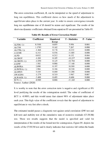
The error correction coefficient, ∅, can be interpreted as the speed of adjustment to
long run equilibrium. This coefficient shows us how much of the adjustment to

equilibrium takes place in the current year. In order to ensure convergence towards
long run equilibrium sine of ∅ should be minus and significant. The results of the

short-run dynamic coefficients obtained from equation 03 are presented in Table 05.

Table 05: Results of Error Correction Model
Variable Coefficient Slandered T - Statistics P - Value
Error
LFDI(-1)) 0.3301 0.055 5.956 0.001
LCTR 1.1783 0.162 7.267 0.000
LCTR(-1)) -1.468 0.178 -8.233 0.000
 LEXR 6.343 0.556 11.405 0.000
LFD 0.032 0.212 0.152 0.884
LGROT -1.281 0.105 -12.237 0.000
LGROT(-1)) -1.850 0.125 -14.784 0.000
 LINF 1.502 0.088 17.160 0.000
LINFRA 2.090 0.197 10.589 0.000
LINFRA(-1)) 1.904 0.186 10.320 0.000
LOPEN 5.418 0.480 11.288 0.000
WAGIN) -1.279 0.319 -3.967 0.007
LWAGI(-1)) -3.488 0.405 -8.606 0.000
ECT(-1) -0.989 0.088 -11.243 0.000
Source: Author (2020)

It is worthy to note that the error correction term is negative and significant at 0%
level justifying the results of the cointegration model. The value of coefficient of

ECT is -0.9893, and this would mean that almost 98% of adjustment takes place

each year. This high value of the coefficient reveals that the speed of adjustment to
equilibrium is very fast after a shock.

The estimated model passes a diagnostic test against serial correlation (DW test and

LM test) and stability test of the cumulative sum of recursive residuals (CUSUM)
test. These test results suggests that the model is specified and valid for

interpretation of the results of the bound test for cointegration. Figure 05. depicts the
results of the CUSUM test and it clearly indicates that statistics fall within the bands

65